7 Statistics
- Deterministic vs stochastic process: a deterministic process is a mathematical model where the output depends solely on the input, and there is no randomness involved. In contrast, a stochastic process is a mathematical model that involves randomness and is used to model situations that may not have inherent randomness. A deterministic model is completely predictable also.
- Unit root is a feature of some stochastic processes. A linear stochastic process has a unit root if 1 is a root of the process’s characteristic equation. Such a process is non-stationary. If the other roots of the characteristic equation lie inside the unit circle, then the first difference of the process will be stationary; otherwise, the process will need to be differenced multiple times to become stationary.
- Bias is a systematic tendency to underestimate or overestimate the value of a parameter (you were not random!). It implies that the data selection may have been skewed by the collection criteria (in favor or against an idea). It can also be defined as a systematic (built-in) error which makes all values wrong by a certain amount. In ML, the inability for a ML method to capture the true relationship is called bias, that happens because algorithm makes simplified assumptions so that it can easily understand the target function.
| Bias | Error |
|---|---|
| Produces prejudiced results | Results in inaccurate outcomes |
| Identified manually or through software packages | Identified through calculations |
| Occurs systematically | Occurs randomly |
- Normal/uniform distribution is the kind of distribution that has no bias either to the left or to the right and is in the form of a bell-shaped curve. In this distribution, mean is equal to the median.
- Skewed distribution is a distribution where the curve is inclined towards one side.
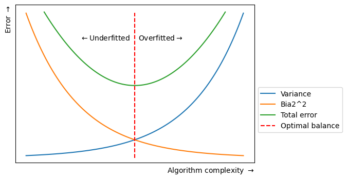
- Variance is a statistical measurement used to determine the average of each point from the mean (the average of the squared differences from the mean). In ML the difference in fits between training and test sets is called variance, i.e. it refers to the changes in the model when using different portions of the training data set. Simply put, variance is the variability in the model prediction. Standard deviation is the spread of a group of numbers from the mean.
\[ Var(X) = E[X^2] – E[X]^2 \]
| Signs of high bias ML model | Signs of high variance ML model |
|---|---|
| Failure to capture data trends | Noise in data set |
| Underfitting | Overfitting |
| Overly simplified | Complexity |
| High error rate | Forcing data points together |
- Robustness represents the system’s capability to handle differences and variances effectively
- Total error = variance + bias + irreducible error
- Correlation vs covariance: correlation is a measure of relationship between two variables and says how strong are the variables related. Range is -1 to 1. Covariance represents the extent to which the variables change together in a cycle. This explains the systematic relationship between pair of variables where changes in one affect changes in another variable. Range is -inf to +inf, and is affected by scalability.
- Confounding variables are extraneous variables in a statistical model that correlates directly or inversely with both the dependent and the independent variable. Left unchecked, confounding variables can introduce many research biases to your work, causing you to misinterpret your results.
- R-squared/coefficient of determination is a statistical measure in a linear regression model that determines the proportion (percentage) of the variance in the dependent variable that can be explained by the independent variable. In other words, it evaluates the scatter of the data points around the fitted regression line, i.e. shows how well the regression model explains observed data.
\[\begin{aligned} R^{2} &= 1 - \frac{\text{Residual variance}}{\text{Total variance}} \\ &=\frac{\text{Total variance - Residual variance}}{\text{Total variance}} \\ &=\frac{\text{Explained variance}}{\text{Total variance}} \\ &=\text{Fraction of total variance explained} \end{aligned}\]
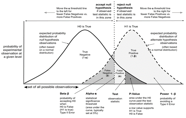
p-value is the measure of the statistical importance of an observation. We compute the p-value to understand whether the given data really describes the observed effect or not. If p<=0.05 it suggests that there is only 5% chance that the outcomes of an experiment are random and the null hypothesis must be rejected. \[ p_{value} = P(E|H_{0}) \]
The statistical power of a binary hypothesis test is the probability that the test rejects the null hypothesis when a specific alternative hypothesis is true
Confidence interval is a range of values likely containing the population parameter. Confidence level is denoted by 1-\(\alpha\), where \(\alpha\) is level of significance (usually 5%). Point estimate is an estimate of the population parameter (can be derived with Maximum Likelihood estimator for egz.)
Univariate, bivariate and multivariate analysis: univariate analysis allows us to understand the data and extract patterns and trends out of it. Bivariate analysis allows us to figure out the relationship between the variables. Multivariate analysis allows us to figure out the effects of all other variables (input variables) on a single variable (the output variable).
Sampling is the selection of individual members or a subset of the population to estimate the characters of the whole population. It is useful with datasets that are too large to efficiently analyze in full. There are two types of sampling techniques: probability and non-probability. Resampling is the process of changing/exchanging data samples, identifying the impact of these changes on model and prediction characteristics, and continuing until optimal results are achieved. It is done in cases of estimating the accuracy of sample statistics or validating models by using random subsets to ensure variations are handled (egz. Bootstraping, cross-validation)
Types of biases that can occur during sampling: selection bias, undercoverage bias and survivorship bias. Selection bias occurs when a sample selection does not accurately reflect the target population. Survivorship bias is the logical error of focusing on aspects that support surviving a process and casually overlooking those that did not. This can lead to wrong conclusions in numerous ways.
Bootstrap method is a resampling method by independently sampling with replacement from an existing sample data with same sample size n, and performing inference among these resampled data.
Normalization/Min-Max scaling is used to transform features to be on a similar scale ([0,1] or [-1,1]). It is useful when there are no outliers. \[ X_{new} = (X - X_{min}) / (X_{max} - X_{min}) \] Normalization is useful when your data have different dimensions and the method you’re employing doesn’t make assumptions about the distirbution of you data.
Standardization/Z-score normalization is the transformation of features by subtracting from mean and dividing by standard deviation. It is not affected with outliers since its not bounded to a certain range. Changing the range of your data with scaling is different from changing the distribution of your data with Normalization. Also, standardization presupposes that the distribution of your data is Gaussian. \[ z = \frac{x-\mu}{\sigma}, \] where \(\mu\) represents the mean and \(\sigma\) represents the standard deviation.
The Central limit theorem says that, given a large enough sample size, the distirbution of sample averages/means will be approximtely normal. This means that we can use normal distirbution to make predictions about populations based on samples.
The Law of large numbers is a theorem that describes the result of performing the same experiment very frequently. It states that the sample mean, sample variance, and sample standard deviation converge to what they are trying to estimate
Gradient, for purposes of this paper, measures how much the output of a function changes if you change the inputs a little bit (from a given point).
Categorical, continuous and ordinal variables. An ordinal variable is a categorical variable for which the possible values are ordered.
Histrograms vs boxplots: Boxplots are more often used in comparing several datasets and take less space than histograms. Histograms are used to know and understand the probability distribution underlying a dataset
Histograms vs bar graphs: a bar graph is the graphical representation of categorical data, whereas a histogram is the graphical representation of data where data is grouped into continuous number ranges
Kernel density estimation (KDE) is a method for visualizing the distirbution of observations in dataset over a continuous interval or time period
Histograms vs density plots: an advantage that density plots have over histograms is that they’re better at determining the distribution shape because they are not affected by the number of bins used.
Akaike information Criterion (AIC): is a mathematical method for evaluating how well a model fits the data it was generated from. In statistics, it is used to compare different possible models (model selection). Lower AIC scores are better!